Neural Networks

Introduction

Part I dealt with neural networks operating with fixed weights. That system works when it is possible to discriminate clearly between inputs and appropriate weights can be found for the network units. A network using learning by back-propagation can adjust weights to improve discrimination when input data is incomplete or noisy.

Weights are adjusted by calculating correction increments from a known input to the net and the desired output and the actual output. The mathematics is given here in revelatory fashion; anyone who wants the dirty detail can find it in Ref.2 for Part I.

The Sigmoid Function

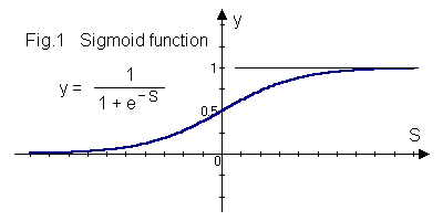
In Part I the output of a unit with fixed weights was found by applying a hardlimiting function to the weighted sum of the inputs. Correction increments for back-propagation are calculated from a derivative of a unit’s output but the hardlimiting function is not continuous and so not differentiable. A continuous, monotonic function, the sigmoid function illustrated at Fig.1, is used instead.

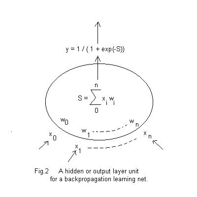
The sigmoid output y of a unit in the hidden or output layer is

where S is the same weighted sum as for a fixed weights unit. That output is, as before, delivered to all output units from a hidden unit or forms part of the network output from the output layer. Each input layer unit still delivers its input unchanged to every hidden layer unit.

The working scheme for a hidden or output unit is now as shown at Fig.2. Notice that binary outputs cannot occur; sigmoid outputs can only tend towards 0 or 1 so in any network application criteria for evaluating such output is needed.

Correction of output unit weights

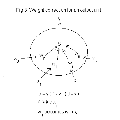
The correction procedure is different for output and hidden units because, initially at least, desired values exist only for the output units. Output layer units are corrected first.

An input for which a desired network output is known is delivered to the network. That input, the hidden layer output and the network output are recorded.

For each output unit an error value

is calculated where y is the unit’s actual output and d is it’s desired output. Then the correction increment for each i’th weight of the unit is

where k is a constant, the learning rate, 0 < k < 1, and x_i is the input to the weight w_i.

The new weight is obtained by adding c_i to the old weight.

Correction of hidden unit weights

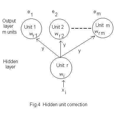
The procedure a hidden unit is as for an output unit except that the error value for a weight is calculated using a weighted sum of all the error values for the output layer. The description below uses the notation shown in Fig.4 where we are working with the i’th weight of the r’th hidden unit and error values e₁ to e_m have been calculated for the m output units.

The weights of the output layer having been adjusted a weighted sum W_r of the error values for the output units is calculated. The weights used are those for the input from hidden unit r, giving

which is used to calculate the error value e_r for hidden unit r,

and the correction increment for the i’th weight of hidden unit r is

where x_i is the input to w_i of unit r and k is the learning constant.

Programs

At this point it would be nice to present a learning program utilising back-propagation but unfortunately that program is not yet reliable. If you want to know why just look back at the last few paragraphs. It will appear, ed willing, in Part III with learning versions of the networks presented in Part I. For now I offer some other programs for back-propagation procedures.

Program ‘PREP’ is the same as the program of that name in Part I except that it controls number format. Enter data at the prompts to set up a net. The numbers of input, hidden and output units are stored as ‘Ino’, ‘Hno’ and ‘Ono’. The weights for hidden and output units are stored as arrays at ‘Hwts’ and ’Owts’ with each unit’s weights as a column vector, unit 1 in the first column, w₀ at the top.

« "PREP" DROP 
RCLF -49 CF -50 CF
"Enter no. inputs" "" INPUT OBJ-> 'Ino' STO
"Enter no. hidden units" "" INPUT OBJ-> 'Hno' STO 
1 Hno FOR j
"Enter weights 0 to " Ino + " for hidden unit " + j + 
"" INPUT OBJ-> NEXT 
Hno 'Ino+1' 2 ->LIST ->ARRY TRN 'Hwts' STO
"Enter no. outputs" "" INPUT OBJ-> 'Ono' STO 
1 Ono FOR j
"Enter weights 0 to " Hno + " for output unit " + j + 
"" INPUT OBJ-> NEXT 
Ono 'Hno+1' 2 ->LIST ->ARRY TRN 'Owts' STO STOF
»

Checksum # 9340h, 468.5 bytes.

Program ‘RUNIT’ operates whatever net has been set up by ‘PREP’. It is the same as the program of the same name in Part I except that it calls the sigmoid function instead of ‘hardlimit’, controls number format and saves layer inputs as row vectors ‘HXi’ and ‘OXi’ for when it is called by the learning program. A layer output is obtained as a row vector by multiplying the row vector of inputs and the array of layer weights. Enter input values at the prompt. Net output values are delivered as a list, using 1 FIX format, with the value from output unit 1 at the head. For more decimal places alter the FIX parameter in the last line.

« "RUNIT" DROP 
-49 CF -50 CF 
1 "Enter inputs 1 to " Ino + "" INPUT 
OBJ-> 1 'Ino+1' 2 ->LIST ->ARRY 
DUP 'HXi' STO
Hwts * sigmoid 
[ 1 ] 1 COL+ 
DUP 'OXi' STO
Owts * sigmoid 
OBJ-> OBJ-> DROP SWAP DROP ->LIST
1 FIX
»

Checksum # 3970h, 242.0 bytes.

Program ‘sigmoid’ is called by ‘RUNIT’. It takes a row vector of layer outputs, disassembles it, rotates the elements on the stack while applying the sigmoid function to each one and then reassembles the vector.

« "sigmoid" DROP 
OBJ-> OBJ-> DROP SWAP DROP -> c
  « 1 c
    START NEG EXP 1 + INV c ROLLD NEXT 
    1 c 2 ->LIST ->ARRY
  »
»

Checksum # 2016h, 95.0 bytes.

Program ‘VYOO’ enables inspection of net elements to see how learning is affecting them. The small screen is a problem. Each row of a weights display shows the weights of one unit in 1 FIX format, the first unit at the top and w₀ at the left. For more decimal places alter the FIX parameter. If an array is too large for the screen then user must recall the matrix and use the matrix writer instead, in which case the weights of units are seen as column vectors, unit 1 at the left, w₀ at the top.

« "VYOO" DROP 
FONT-> FONT6 ->FONT -49 -50 CF CF CLLCD
"Net configuration -"
Ono + " output units, " + 
Hno + " hidden units, " +
Ino + " input units." + 3 DISP 
{ { "NEXT" « CONT » } } TMENU 
7 FREEZE -1 WAIT DROP 
1 FIX CLLCD
“Last hidden input;” 3 DISP HXi sho 4 DISP
“Last output input;” 6 DISP OXi sho 7 DISP
7 FREEZE HALT CLLCD
"Hidden weights -" 1 DISP Hwts unrap
7 FREEZE HALT
CLLCD
"Output weights -" 1 DISP Owts unrap
7 FREEZE HALT STOF ->FONT 
{ { “FINIS” « 2 MENU » } { “AGAIN” « VYOO » } } TMENU
»

Checksum # 23DCh, 529.0 bytes.

Program ‘sho’ is called by ‘VYOO’ to display layer input values as lists.

« “sho” DROP OBJ-> OBJ-> DROP SWAP DROP ->LIST »

Checksum # B08Ah, 35.5 bytes.

Program ‘unrap’ is called by ‘VYOO’ to display layer weights.

« “unrap” DROP TRN OBJ-> OBJ-> DROP -> r c
  « r 1 FOR R ->STR 1. 'c-1'
          START " " SWAP + + NEXT 
      c R 1. - * 1 + ROLLD -1 STEP 
    1 r
    FOR R R 1 + DISP
    NEXT
  »
»

Checksum # 133h, 158.5 bytes.

The source code for the programs in this article can be downloaded from Peter Gatenby’s web site at http://www.freenetpages.co.uk/hp/pvg or HPCC’s web site here